
The Australian Bureau of Statistics recently announced that Australia’s inflation rate for the 12 months to the end of March 2022 was 5.1%, the highest rate since the introduction of the Goods and Services Tax in 2000. In the US, inflation for the same period rose 8.5%. Consequently, it is now widely accepted that inflationary forces are not transitory, and the global economy has entered a period of rising prices.
In response to these very high price increases it is expected that central banks will increase interest rates until inflation is brought down. Investors are now examining their portfolios to understand how these two economic forces (increasing prices and increasing interest rates) will impact their investments. This article will examine how these two forces may impact the Rural Funds Group (ASX: RFF) and the 18,000 investors who hold this investment in their portfolios.
Rising prices
To gain an understanding of how inflation will impact the performance of agricultural assets, it is useful to look at the history of previous inflationary periods. Although history cannot be used to predict the future, it will at least provide a feel for the likely duration and amplitude of what might happen.
Figure 1 presents data from the past 120 years, by plotting the movement in US commodity prices and inflation for both the US and Australia. The data is presented by plotting the data over rolling ten-year periods to smooth annual volatility and make distinct periods more discernible. During the period, both the US and Australia, and for that matter all developed economies, experienced three very similar periods of high inflation, with what may be a fourth period occurring now. Notably, during the three earlier periods, commodity prices followed the same course as inflation, which is unsurprising, since inflation indices are in a large part the measure of the change in the price of goods which are manufactured from commodities.
Figure 1: US All Commodities prices, Australian Inflation and US Inflation rates1

Understanding the history of what drove these periods of high inflation is useful because we can then consider if any of these factors are present now. Furthermore, understanding how these factors were managed, may provide some guide as to what measures will be taken to slow the current rate of increasing prices.
The first wave of rising prices occurred from 1897 to 1920 and was a consequence of the industrialisation of western economies. New technologies such as electrical power stations, telephones and cars were rapidly deployed, creating new jobs in manufacturing and a mass migration of poor rural workers to the cities, in a great wave of urbanisation. Prices then rocketed with the outbreak of World War I, with the disruption of food production in the battlefields of Europe and the increased demand for food and weapons.
When peace finally came in 1918, European food production began to recover. Demobilisation created high levels of unemployment, so that by 1920, the global economy entered a period of declining commodity prices, low wages growth and consequently lower rates of inflation. A significant contributing factor to this turning point was a change in direction of US monetary policy with accommodative war time interest rates of 4% increasing to 7% between December 1919 and June 1920.
The second wave of rising prices from 1933 to 1951, began with another change in monetary policy when as a consequence of the Great Depression (1929-1933), countries elected to leave the gold standard so they could pursue expansionary monetary policies. Among the first to leave were Australia and Canada in December 1929, then in 1933, the US, by far the world’s largest holder of gold, raised its conversion price of gold from USD20.67 to USD35.00 per ounce, which effectively increased that country’s stock of money.
From that point on, world economies began to recover, with demand and consequently prices rising once more until the outbreak of World War II in 1939. Demand for commodities once again soared as US government spending expanded from 10% of GDP in 1940 to 46% by 1943, then held at 40% for the following two years. Post war, high rates of government spending continued, while interest rates were kept low due to pressure brought to bear on the US Federal Reserve, by the US Treasury.
The turning point for this period of high inflation, came in 1951 when there were major changes to monetary policy. In March 1951, the US Treasury-Federal Reserve Accord was announced, to define and separate the roles the US Treasury and the Fed. Three weeks later the President announced a new Fed Chairman, and the tightening of monetary policy began.
The third wave of rising prices occurred during the period 1968 to 1981 and was initially caused by debt funded spending by a government reluctant to raise taxes to fund the unpopular Vietnam War. During the ten years to 1975, US government debt doubled, which increased the supply of money. In 1971, confidence in the US dollar was eroding and in response to this, President Nixon abandoned the Bretton Woods agreement which enabled convertibility of US dollars into gold. This effectively floated the US currency and caused a depreciation against other major currencies.
This chain of events was followed by a decision by major oil producers though OPEC, to price oil off the value of gold, sending US dollar oil prices higher. Then in 1973, Arab oil producers embargoed supplies of oil to the US and other Western nations due to their support for Israel during the Yom Kippur War. This sequence of events caused oil to rise from USD3.00 per barrel in 1972 to USD37.00 by 1980. This caused US inflation to average 9.4% per annum from 1974 to 1981.
Once again, a change in monetary policy following the appointment of Paul Volcker as chairman of the US Federal Reserve, creating the next turning point. Volcker immediately set about tightening money supply and increasing interest rates, with the federal funds rate rising from 11% in 1979 to 20% in June 1981.
There are some common themes among these three inflationary periods that may have some similarities with the current period of rising prices. In the first two waves, robust demand from growing economies was then super charged by war-spending funded by government debt that increased money supply. In the third wave, war came first and a trade war second. In all cases, the actions taken by government treasuries and central banks initially fed rising prices. Then, with changes of policy direction, through tightening of the supply of money, inflation was reined in.
In more recent times, governments and their central banks intervened to support economic activity in response to the global financial crisis which began in 2007.
Accommodative monetary policy continued for many years following the crisis. Then this was followed by the response to the COVID-19 pandemic, which has increased the stock of money in the global economy by trillions of dollars. With these actions supporting demand, interruptions in supply chains have caused shortages across many sectors. This has resulted in an increase in the price of commodities and the goods manufactured from them. These increases are now being recorded and reported in inflation statistics.
Rising land values
Having gained an understanding of the factors driving inflation, it is now time to consider the implications of these cycles on agricultural land values. Figure 2 once again presents the long-term movement in commodity prices, a basket of basic goods that includes sub-categories such as energy, metals and agricultural commodities. Agricultural commodities are separately presented to demonstrate the high correlation that exists between agriculture and the broader commodities index.
Figure 2: US Energy and Metals Commodities and US Agricultural Commodities prices2

Figure 3 represents agricultural commodity price movements alongside the change in value of US and Australian farmland. As can be seen, the rate of change in farm values closely follows the waves in agricultural commodity prices, which is to be expected, given farm profits are largely determined by the price that producers are paid for the commodities they grow. While the available Australian data is shorter term, the correlation with commodity prices is still apparent.
It should be noted that lines that describe farmland and commodity price movements are not the outright price, but instead the percentage change in price. In the chart, it is evident that US farm values experienced two periods of outright price decline with the first and most severe spanning the period 1920 to 1933. Throughout the balance of this 120-year period, farm values have experienced periods of modest gains and periods of high growth that generally coincide with periods of increasing commodity prices.
Figure3: US Agricultural Commodities, US Farmland prices and Australian Farmland3

One curious period in Figure 3 is from 1951 to 1968, when outright agricultural commodity prices declined by 12.5%, but farm values increased by approximately 140%. This can be explained by the productivity gains achieved by American farmers as they mechanised their operations, applied new synthetic fertilisers and grew better plant varieties. During the 1950s the number of hired workers on American farms declined by 30%, while tractor sales reached 600,000 per year, and land previously used to feed the horses that powered farm operations was turned over to producing higher volumes of grain.
Crop yields also rose, with wheat yields in tonnes per hectare for the US increasing from 1.1 to 1.9, corn yields increased from 2.3 to 5.0 and soybeans from 1.4 to 1.8 tonnes per ha. It is productivity gains such as these, that sustain capital growth in agricultural land values over a full inflationary cycle.
In the past decade agricultural commodity prices have been rising and farm values as well. In Australia, farm values rose at a modest pace in the decade following the Global Financial Crisis, while over the past two years values have probably increased between 20% to 50%. Higher gains have occurred in the grazing and cropping industries where conditions have been particularly favourable. Liquidity has also been a significant factor in driving recent gains, with better access to finance for working capital and the weight of funds from foreign investors particularly from North America.
The Rural Funds Group
The Rural Funds Group (ASX: RFF), buys farms generally using bank debt equal to 35% of the farms value, because debt is cheaper than equity. In fact, debt has been very cheap recently, with variable interest for farm loans costing around 1.56%.4 However, it now appears that interest rates are rising and this will impact the net profits of the fund. RFF has, however, hedged or effectively fixed 42% of its term debt,5 which means that a 1% increase in interest rates based on current debt,5 would increase interest expenses by $2.53m per annum.6
This increased cost can, however, be offset by the increase in rental income from the assets that are leased. As an investor in agricultural land and water entitlements, RFF has been a beneficiary of the recent favourable price movements. Over the past five years, RFF's vineyard values have increased by 47%,7 although this sector is currently challenged by very high tariffs now imposed in the once fast-growing Chinese market. Almond prices have declined in the last seven years due to large crops produced by the dominant US industry. Despite this, the fund’s almond orchards values have increased 22% over the period.7 The value of RFF’s cropping assets has increased by 15% and cattle assets by 98%.7 Water licence values have also increased during the period by 91%.7
Increased assets values are a handy thing for RFF, since they increase the net assets of the fund and therefore the amount of equity held by the fund to finance its investment activities.
Over time increasing asset values and inflation also transmit to the amount of cash income generated by the fund from rents because of the rental indexation mechanisms contained in the agreements RFF has with its lessees. Of the leases 44% are indexed to CPI and 34% have fixed annual increases, but with a review to the market value of the farm every five years.8 In total, 82% of RFF’s leases provide rental indexation that occurs as a result of land value changes or inflation.8 Importantly, a period of rising commodity prices is of great benefit to RFF’s lessees as they generate higher profits from the commodities that they produce.
Conclusion
Having considered the history of previous inflationary cycles and the actions taken by government and central banks, it is apparent that the national economies of the world recently experienced, and indeed created, very similar inflationary conditions. It is also now evident that central banks at the very least, have now begun the necessary task of reducing inflation, by increasing interest rates.
Agricultural commodity prices have typically risen during periods of inflation, then declined during periods of rising interest rates. Concurrently, farm values have risen during periods of inflation and experienced generally brief periods of price declines as interest rates have risen. For this reason, as we enter the end phase of this inflationary cycle, it is probable that farm values will not increase as they have most recently done so. In our view, RFF’s values will most probably not decline either, due to ongoing productivity gains.
Over the next few years RFF will likely experience higher interest rates on its debt, while accruing increased rents from higher inflation and recently increased land values. Longer term, RFF will need to continue to identify and develop productivity gains across its portfolio of assets, so that increased profits can be shared between landlord and lessee. History shows us that cycles are unavoidable, but progress through productivity is possible.
Notes:
- Graph shows the ten-year moving average of percentage change. US All Commodities includes US energy, metals and agricultural commodities. Source Federal Reserve Economic Data (FRED) St. Louis Fed (stlouisfed.org) and Australian Bureau of Statistics (ABS).
- Graph shows the ten-year moving average of percentage price change. Source Federal Reserve Economic Data (FRED) St. Louis Fed (stlouisfed.org).
- Graph shows the ten-year moving average of percentage price change. Source Federal Reserve Economic Data (FRED) St. Louis Fed (stlouisfed.org) and the Australian Bureau of Agricultural and Resource Economics and Sciences (ABARES).
- Based on an estimate of RFF’s forecast unhedged cost of debt for FY22.
- RFF’s term debt as at 31 December 2021.
- Calculated based on an assumed increase in interest rates by 1% on the unhedged term debt balance at 31 December 2021.
- Percentage increases subject to rounding and are calculated only on assets in each agricultural sector which were owned (and mature in the case of almond orchards) on 31 December 2016 through to 31 December 2021. The increase in values are calculated as the percentage movement between 2016 and 2021 encumbered valuations adjusting for capex. Water license values relate to assets not included in property leases.
- Percentage increases subject to rounding and based on FY22f revenue by lessee type, as per RFF HY22 financial results.